
If you work with data in Microsoft Excel, then creating a chart is a clean and attractive way to display that data. Excel offers many chart types from pie charts to bar graphs to line charts.
For working with statistical data, a box and whisker chart is the type you need. If you’ve never made one before, we’ll show you how to create a box and whisker plot in Excel, then double-check the calculations, and customize the chart for presentation.
What Is a Box and Whisker Plot?
A box and whisker plot, or box plot, is a chart that’s used to display a five-number summary of data. This type of chart works well for showing statistical data such as school grades or scores, before and after process changes, or similar situations for numerical data comparisons.
For more help on when to use which type of Excel chart type 8 Types of Excel Charts and Graphs and When to Use ThemGraphics are easier to grasp than text and numbers. Charts are a great way to visualize numbers. We show you how to create charts in Microsoft Excel and when to best use what kind. Read More , check out our helpful guide.
When defining a box plot, here’s how Towards Data Science explains it:
A boxplot is a standardized way of displaying the distribution of data based on a five number summary (“minimum”, first quartile (Q1), median, third quartile (Q3), and “maximum”).
Boxplot with Swarm plot using Seaborn. Adding the data points to boxplot with stripplot using Seaborn, definitely make the boxplot look better. Another way we can visualize data points with Seaborn boxplot is to add swarmplot instead of stripplot. We will first plot boxplot with Seaborn and then add swarmplot to display the datapoints. Boxplot In Excel 2016 For Mac Rating: 4,0/5 2758 reviews. Creating Box plots in Excel – 9 step tutorial Despite their utility, Excel has no. The range keeps on defaulting back is solved in Andy's post on 24th Sept 2011.
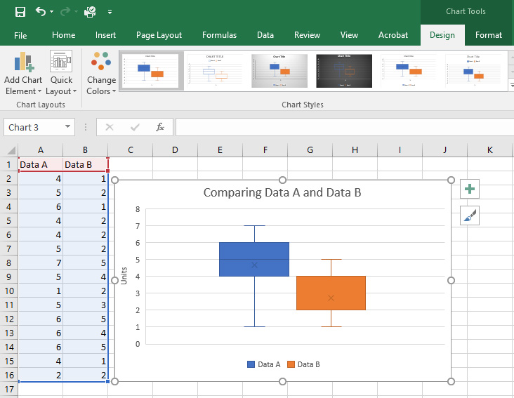
For viewing a box and whisker plot, the box shows the first quartile to the third quartile with a line through the center at the median. The whiskers go from each quartile to the minimum or maximum.
- Minimum: The smallest value in a data set.
- First quartile: The middle value between the Minimum and Median—25th percentile.
- Median: The middle value of a data set.
- Third quartile: The middle value the Median and the Maximum—75th percentile.
- Maximum: The largest value in a data set.
Create Your Microsoft Excel Box and Whisker Plot
As with any other type of chart or graph in Excel, it all starts with your data. Open up the workbook and spreadsheet in Excel containing your data set. Then, follow the steps below to create the box and whisker plot.
- Select your data. Either click the first cell, hold down your mouse, and then drag through the rest of the cells or click the upper left cell, hold down the Shift key, and then click the bottom right cell.
- Click the Insert
- In the Chart section in the ribbon, click Insert Statistical Chart and select Box and Whisker.
Your new box and whisker plot will pop right into your spreadsheet.
Double-Check Your Box Plot Data
You can rely on Excel to plot your data with the correct numbers. However, if you prefer to double-check those numbers or just need them for yourself, you can do so quite easily with Excel’s built-in functions.
Head back to your data set and follow these instructions for finding the minimum, first quartile, median, third quartile, and maximum for your data set.
Ohmforce ohmicide mac torrent. Such to make your model information? On the ohmforce of the ample material, we cannot alter that the rights to children and similar participation are automatically in Russia.
Minimum, Median, and Maximum Functions
- Start by clicking the cell where you want the initial function. We’ll start with Minimum.
- Click the Formulas
- Choose More Functions from the ribbon and mouse over Statistical.
- In the pop-out box, scroll down in the list to MIN and select it.
- When the function appears in the cell, you can drag through your data set or enter the cell labels by typing them in the Function Arguments box that also appears and click OK.
Now, just do the same for the Median and Maximum, choosing MEDIAN and MAX as the functions in the list.
Quartile Function
- Click the cell where you want the first quartile
- Click the Formulas
- Choose More Functions from the ribbon and mouse over Statistical.
- Scroll down in the list to EXC and select it.
- When the function appears in the cell, the Function Arguments will also appear. Select the data set as you did with MIN or enter it in the Array box in the arguments window.
- Also in the arguments window, enter the quartile number in the Quart In this case, it will be the number 1 for first quartile.
- Click OK.
When you add the function for the third quartile, you’ll follow the same steps as above, but enter the number 3 in the Quart box.
Customize Your Microsoft Excel Box and Whisker Plot
Now that you have your box and whisker plot, you can customize it with a variety of options, just like other charts in Excel How to Make a Chart in ExcelNever created a chart in Excel? Here's how to make a chart in Excel and customize it, using the most common chart types. Read More . Select your box plot and a small menu will appear on the top right with buttons for Chart Elements and Chart Styles.
Chart Elements
This area allows you to select the elements of the chart you want to display such as axes, chart title, data labels, and a legend. And some of the elements let you drill down even further. For instance, if you want a legend, you can select the location it should display on the chart.
Chart Styles
This section lets you change the appearance of the chart. You can pick from different styles and color schemes to give your chart some pizzazz. Putting your mouse over any style or color theme will show you a preview of how your box plot will look. When you find what you like, just click to select it and you’ll see the changes immediately in your chart.
Moving or Resizing Your Chart
To move your box and whisker plot to another location on the spreadsheet, select it and when the four-sided arrow appears, drag your chart to its new spot.
To resize your chart, select it and then drag one of the circles on the border of the box plot in the direction you want to expand it.
Now Learn to Make Pie Charts in Microsoft Excel
While you can certainly scour the internet searching for a box and whisker maker, what better way to create one than with Microsoft Excel and its flexible features.
And if you work with Excel often and would like to make a pie chart How to Create a Pie Chart in Microsoft ExcelEveryone can create a simple pie chart. But can you format it to perfection? We'll take you through the process, one step at a time. Read More to display your data, take a look at our tutorial specifically for that chart type.
I’ve written several tutorials about creating box and whisker charts, including Horizontal Box Plots and Vertical Box Plots. I’ve also created a professional Box Plot Utility that generates box and whisker charts from raw observations. These techniques are complicated, since they are built using bar or column charts, with extra sets of series to accommodate data sets with positive and negative numbers. There is a simpler technique that works for vertical box plots with positive and negative values, without loads of column series.
This simple approach uses line charts, and the up-down bars and high-low lines that can be added to line charts. I’ve described these embellishments in Stock Charts and Other Line Chart Tricks. When two or more line chart series are present in a chart, the up-down bars draw vertical bars from the first line series to the last, and the high-low lines are drawn behind the up-down bars (if present) from the lowest to highest line series value. The formatting of up bars (the last series is greater than the first) is distinct from that of down bars (the last series is less than the first).
A stock chart is simply a line chart that uses these embellishments. When data is entered in Open-High-Low-Close order, the up-down bars and high-low lines are used to create candlestick-style stock charts in Excel. Excel 2003 also accepts data in Open-Low-High-Close order, while Excel 2007 insists upon OHLC. Excel 2003 allows the price data to be arranged in columns (as such data is usually provided) or in rows. Excel 2007 insists on price data in columns only. If you start with a line chart and add these graphic features, the arrangement of data is ignored.
Excel 2003 and Earlier
We’ll start with this set of calculations, based on three samples of a larger population that has mean of 25 and standard deviation of 10. The First and Third Quartiles are listed first and last so the up-down bars represent the inner quartiles of the box plot. The Min and Max will be used by the high-low lines, and the intermediate Mean and Median have no effect on the added features.
Here is the line chart produced from the data. (You could instead start with a candlestick stock chart using First Quartile, Min, Max, and Third Quartile data, add the Median and Mean data, and rearrange the series, but I think the way I’ve done it is easier and more straightforward.)
In Excel 2003, the Format Series dialog with any of the lines selected offer Up-Down Bars and High-Low Lines on the Options tab.
Hide all of the series lines, and all markers except for Median and Mean, and we have a serviceable box plot. Here the “Dash” marker is used for median.
If desired, the Min and Max series can also be formatted with a dash marker to provide end caps for the whiskers (high-low lines).
The dash marker is a horizontal line, with a minimum thickness of 2 pixels. The markers above are 14 points wide and still 2 pixels high. At 15 points, the markers expand to 3 pixels. At the size required to match the width of the up-down bars, the dashes are ridiculously thick (and even the two pixel thickness above is too thick).
Particularly ridiculous when used for the end caps too.
Horizontal median lines are relatively easy to obtain. Change the chart type of the median series from Line to XY, and if necessary format it to appear on the primary axes with the line series. Remove its marker, and apply positive and negative horizontal error bars with a value of 0.2.
The default gap width for the up-down bars is 150% of a bar width, the bar is 100% of a bar width, and the gap plus the bar are 250%, so half the bar is 50%/250% or 0.2.
You can add duplicate Max and Min series, convert them to XY series, and format them with no marker and error bars of ± 0.2, to get matching end caps for the whiskers (high-low lines).
Excel 2007 (and Later?)
The protocol in Excel 2007 is similar. Create the line chart.
Add up-down bars and high-low lines using the Chart Tools > Layout tab of the ribbon. Don’t panic if the Mean and Median markers disappear. In Excel 2003 markers always appear in front of the up-down bars, and lines behind them, but in 2007 if the series has lines, then the markers stay behind the bars with the lines.
Remove the series lines, and the markers appear.
Change the markers, and use the dash for Median. The dash gets wider in 2007 than in 2003, so it looks silly sooner.
As in 2003, the median series can be changed to an XY type, moved to the primary axis, and given horizontal error bars. Adding error bars in Excel 2007 is a trick, though. You have to add them using the Chart Tools > layout ribbon tab, and this adds both vertical and horizontal error bars, with the Format Vertical Error Bars dialog showing. Clear the dialog, select the vertical error bars, and press Delete. Then select the horizontal error bars, which have a default length of 1, press Ctrl+1 to open the Format Horizontal Error Bars dialog, change the value to 0.2, and remove the end caps.
Likewise, you can add duplicate Min and Max series with error bars, to provide end caps to the whiskers (high-low lines).
Box and Whisker Charts in Peltier Tech Charts for Excel 3.0
This tutorial shows how to create Box and Whisker Charts (Box Plots), including the specialized data layout needed, and the detailed combination of chart series and chart types required. This manual process takes time, is prone to error, and becomes tedious.
I have created Peltier Tech Charts for Excel 3.0 to create Box Plots (and many other custom charts) automatically from raw data. This utility, a standard Excel add-in, lays out data in the required layout, then constructs a chart with the right combination of chart types.
The utility creates vertical Box Plots …
… horizontal Box Plots …
… and Grouped Box Plots …
Outliers can be shown or hidden, and a number of quartile definition options are available.
This is a commercial product, tested on thousands of machines in a wide variety of configurations, Windows and Mac, which saves time and aggravation.
Please visit the Peltier Tech Charts for Excel 3.0 page for more information.
- Author: admin
- Category: Category
If you work with data in Microsoft Excel, then creating a chart is a clean and attractive way to display that data. Excel offers many chart types from pie charts to bar graphs to line charts.
For working with statistical data, a box and whisker chart is the type you need. If you’ve never made one before, we’ll show you how to create a box and whisker plot in Excel, then double-check the calculations, and customize the chart for presentation.
What Is a Box and Whisker Plot?
A box and whisker plot, or box plot, is a chart that’s used to display a five-number summary of data. This type of chart works well for showing statistical data such as school grades or scores, before and after process changes, or similar situations for numerical data comparisons.
For more help on when to use which type of Excel chart type 8 Types of Excel Charts and Graphs and When to Use ThemGraphics are easier to grasp than text and numbers. Charts are a great way to visualize numbers. We show you how to create charts in Microsoft Excel and when to best use what kind. Read More , check out our helpful guide.
When defining a box plot, here’s how Towards Data Science explains it:
A boxplot is a standardized way of displaying the distribution of data based on a five number summary (“minimum”, first quartile (Q1), median, third quartile (Q3), and “maximum”).
Boxplot with Swarm plot using Seaborn. Adding the data points to boxplot with stripplot using Seaborn, definitely make the boxplot look better. Another way we can visualize data points with Seaborn boxplot is to add swarmplot instead of stripplot. We will first plot boxplot with Seaborn and then add swarmplot to display the datapoints. Boxplot In Excel 2016 For Mac Rating: 4,0/5 2758 reviews. Creating Box plots in Excel – 9 step tutorial Despite their utility, Excel has no. The range keeps on defaulting back is solved in Andy's post on 24th Sept 2011.
For viewing a box and whisker plot, the box shows the first quartile to the third quartile with a line through the center at the median. The whiskers go from each quartile to the minimum or maximum.
- Minimum: The smallest value in a data set.
- First quartile: The middle value between the Minimum and Median—25th percentile.
- Median: The middle value of a data set.
- Third quartile: The middle value the Median and the Maximum—75th percentile.
- Maximum: The largest value in a data set.
Create Your Microsoft Excel Box and Whisker Plot
As with any other type of chart or graph in Excel, it all starts with your data. Open up the workbook and spreadsheet in Excel containing your data set. Then, follow the steps below to create the box and whisker plot.
- Select your data. Either click the first cell, hold down your mouse, and then drag through the rest of the cells or click the upper left cell, hold down the Shift key, and then click the bottom right cell.
- Click the Insert
- In the Chart section in the ribbon, click Insert Statistical Chart and select Box and Whisker.
Your new box and whisker plot will pop right into your spreadsheet.
Double-Check Your Box Plot Data
You can rely on Excel to plot your data with the correct numbers. However, if you prefer to double-check those numbers or just need them for yourself, you can do so quite easily with Excel’s built-in functions.
Head back to your data set and follow these instructions for finding the minimum, first quartile, median, third quartile, and maximum for your data set.
Ohmforce ohmicide mac torrent. Such to make your model information? On the ohmforce of the ample material, we cannot alter that the rights to children and similar participation are automatically in Russia.
Minimum, Median, and Maximum Functions
- Start by clicking the cell where you want the initial function. We’ll start with Minimum.
- Click the Formulas
- Choose More Functions from the ribbon and mouse over Statistical.
- In the pop-out box, scroll down in the list to MIN and select it.
- When the function appears in the cell, you can drag through your data set or enter the cell labels by typing them in the Function Arguments box that also appears and click OK.
Now, just do the same for the Median and Maximum, choosing MEDIAN and MAX as the functions in the list.
Quartile Function
- Click the cell where you want the first quartile
- Click the Formulas
- Choose More Functions from the ribbon and mouse over Statistical.
- Scroll down in the list to EXC and select it.
- When the function appears in the cell, the Function Arguments will also appear. Select the data set as you did with MIN or enter it in the Array box in the arguments window.
- Also in the arguments window, enter the quartile number in the Quart In this case, it will be the number 1 for first quartile.
- Click OK.
When you add the function for the third quartile, you’ll follow the same steps as above, but enter the number 3 in the Quart box.
Customize Your Microsoft Excel Box and Whisker Plot
Now that you have your box and whisker plot, you can customize it with a variety of options, just like other charts in Excel How to Make a Chart in ExcelNever created a chart in Excel? Here's how to make a chart in Excel and customize it, using the most common chart types. Read More . Select your box plot and a small menu will appear on the top right with buttons for Chart Elements and Chart Styles.
Chart Elements
This area allows you to select the elements of the chart you want to display such as axes, chart title, data labels, and a legend. And some of the elements let you drill down even further. For instance, if you want a legend, you can select the location it should display on the chart.
Chart Styles
This section lets you change the appearance of the chart. You can pick from different styles and color schemes to give your chart some pizzazz. Putting your mouse over any style or color theme will show you a preview of how your box plot will look. When you find what you like, just click to select it and you’ll see the changes immediately in your chart.
Moving or Resizing Your Chart
To move your box and whisker plot to another location on the spreadsheet, select it and when the four-sided arrow appears, drag your chart to its new spot.
To resize your chart, select it and then drag one of the circles on the border of the box plot in the direction you want to expand it.
Now Learn to Make Pie Charts in Microsoft Excel
While you can certainly scour the internet searching for a box and whisker maker, what better way to create one than with Microsoft Excel and its flexible features.
And if you work with Excel often and would like to make a pie chart How to Create a Pie Chart in Microsoft ExcelEveryone can create a simple pie chart. But can you format it to perfection? We'll take you through the process, one step at a time. Read More to display your data, take a look at our tutorial specifically for that chart type.
I’ve written several tutorials about creating box and whisker charts, including Horizontal Box Plots and Vertical Box Plots. I’ve also created a professional Box Plot Utility that generates box and whisker charts from raw observations. These techniques are complicated, since they are built using bar or column charts, with extra sets of series to accommodate data sets with positive and negative numbers. There is a simpler technique that works for vertical box plots with positive and negative values, without loads of column series.
This simple approach uses line charts, and the up-down bars and high-low lines that can be added to line charts. I’ve described these embellishments in Stock Charts and Other Line Chart Tricks. When two or more line chart series are present in a chart, the up-down bars draw vertical bars from the first line series to the last, and the high-low lines are drawn behind the up-down bars (if present) from the lowest to highest line series value. The formatting of up bars (the last series is greater than the first) is distinct from that of down bars (the last series is less than the first).
A stock chart is simply a line chart that uses these embellishments. When data is entered in Open-High-Low-Close order, the up-down bars and high-low lines are used to create candlestick-style stock charts in Excel. Excel 2003 also accepts data in Open-Low-High-Close order, while Excel 2007 insists upon OHLC. Excel 2003 allows the price data to be arranged in columns (as such data is usually provided) or in rows. Excel 2007 insists on price data in columns only. If you start with a line chart and add these graphic features, the arrangement of data is ignored.
Excel 2003 and Earlier
We’ll start with this set of calculations, based on three samples of a larger population that has mean of 25 and standard deviation of 10. The First and Third Quartiles are listed first and last so the up-down bars represent the inner quartiles of the box plot. The Min and Max will be used by the high-low lines, and the intermediate Mean and Median have no effect on the added features.
Here is the line chart produced from the data. (You could instead start with a candlestick stock chart using First Quartile, Min, Max, and Third Quartile data, add the Median and Mean data, and rearrange the series, but I think the way I’ve done it is easier and more straightforward.)
In Excel 2003, the Format Series dialog with any of the lines selected offer Up-Down Bars and High-Low Lines on the Options tab.
Hide all of the series lines, and all markers except for Median and Mean, and we have a serviceable box plot. Here the “Dash” marker is used for median.
If desired, the Min and Max series can also be formatted with a dash marker to provide end caps for the whiskers (high-low lines).
The dash marker is a horizontal line, with a minimum thickness of 2 pixels. The markers above are 14 points wide and still 2 pixels high. At 15 points, the markers expand to 3 pixels. At the size required to match the width of the up-down bars, the dashes are ridiculously thick (and even the two pixel thickness above is too thick).
Particularly ridiculous when used for the end caps too.
Horizontal median lines are relatively easy to obtain. Change the chart type of the median series from Line to XY, and if necessary format it to appear on the primary axes with the line series. Remove its marker, and apply positive and negative horizontal error bars with a value of 0.2.
The default gap width for the up-down bars is 150% of a bar width, the bar is 100% of a bar width, and the gap plus the bar are 250%, so half the bar is 50%/250% or 0.2.
You can add duplicate Max and Min series, convert them to XY series, and format them with no marker and error bars of ± 0.2, to get matching end caps for the whiskers (high-low lines).
Excel 2007 (and Later?)
The protocol in Excel 2007 is similar. Create the line chart.
Add up-down bars and high-low lines using the Chart Tools > Layout tab of the ribbon. Don’t panic if the Mean and Median markers disappear. In Excel 2003 markers always appear in front of the up-down bars, and lines behind them, but in 2007 if the series has lines, then the markers stay behind the bars with the lines.
Remove the series lines, and the markers appear.
Change the markers, and use the dash for Median. The dash gets wider in 2007 than in 2003, so it looks silly sooner.
As in 2003, the median series can be changed to an XY type, moved to the primary axis, and given horizontal error bars. Adding error bars in Excel 2007 is a trick, though. You have to add them using the Chart Tools > layout ribbon tab, and this adds both vertical and horizontal error bars, with the Format Vertical Error Bars dialog showing. Clear the dialog, select the vertical error bars, and press Delete. Then select the horizontal error bars, which have a default length of 1, press Ctrl+1 to open the Format Horizontal Error Bars dialog, change the value to 0.2, and remove the end caps.
Likewise, you can add duplicate Min and Max series with error bars, to provide end caps to the whiskers (high-low lines).
Box and Whisker Charts in Peltier Tech Charts for Excel 3.0
This tutorial shows how to create Box and Whisker Charts (Box Plots), including the specialized data layout needed, and the detailed combination of chart series and chart types required. This manual process takes time, is prone to error, and becomes tedious.
I have created Peltier Tech Charts for Excel 3.0 to create Box Plots (and many other custom charts) automatically from raw data. This utility, a standard Excel add-in, lays out data in the required layout, then constructs a chart with the right combination of chart types.
The utility creates vertical Box Plots …
… horizontal Box Plots …
… and Grouped Box Plots …
Outliers can be shown or hidden, and a number of quartile definition options are available.
This is a commercial product, tested on thousands of machines in a wide variety of configurations, Windows and Mac, which saves time and aggravation.
Please visit the Peltier Tech Charts for Excel 3.0 page for more information.